Group Sequential Design (GSD)
Planning and design
Appropriateness
1) What are the costs of stopping early?
2) Interpreting studies which stop early
- seasonality: is the trial period done in a time frame which is favourable or unfavourable to the effect of the treatment? Would it work as well had it covered extended periods (e.g., both cold and warm seasons)?
- learning effect: did the trial end for futility before the trial team were fully versed in its delivery?
- follow-up duration: are the outcomes measured over a period long enough to convince readers of the value of the findings?
- baseline imbalances: are baseline prognostic factors imbalanced at interim analyses, especially when interim sample sizes are small and what are the potential impact on the results?
3) Will the interim data be ready in time?
4) Are interim data sufficient to inform early stopping?
In context
We encourage PANDA users to read this blogpost 3 summarising issues around early stopping of this trial for efficacy.
References
2. Barnette et al. Oral Sabizabulin for high-risk, hospitalized adults with COVID-19: Interim Analysis. NEJM Evid. 2022;1.
Design concepts
- the criteria researchers wish to stop the trial early for (e.g., futility only, efficacy only, either futility or efficacy, non-inferiority, etc);
- the appropriate stopping rules for making early trial stopping decisions;
- measures of treatment effect (and when this is observed is important to inform early stopping);
- how many times interim data will be analysed (frequency of interim analyses);
- when will interim data be analysed (timing of interim analyses).
Figure 1.
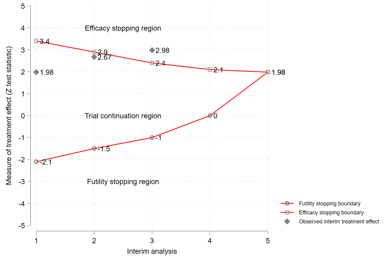
Example of a group sequential design with options to stop early for efficacy or futility. Note: cannot reject H0 and reject H0 could mean that no treatment difference has been established (or new treatment could be worse than the comparator) and researchers have concluded that the new treatment is better (more beneficial) than the comparator, respectively.
Prospective case studies
1. MAPAC trial 4
2. REBOA trial 8,9
References
2. Sato et al. Practical characteristics of adaptive design in phase 2 and 3 clinical trials. J Clin Pharm Ther. 2017; 43(2) :1–11.
3. Todd et al. Interim analyses and sequential designs in phase III studies. Br J Clin Pharmacol. 2001;51(5):394–9.
4. Tröger et al. Viscum album [L.] extract therapy in patients with locally advanced or metastatic pancreatic cancer: a randomised clinical trial on overall survival. Eur J Cancer. 2013;49(18):3788–97.
5. Lan et al. Discrete sequential boundaries for clinical trials. Biometrika. 1983;70(3):659–63.
6. O’Brien et al. A multiple testing procedure for clinical trials. Biometrics. 1979;35(3):549–56.
8. Jansen et al. Bayesian clinical trial designs: Another option for trauma trials? Journal of Trauma and Acute Care Surgery. 2017;83(4): 736–41.
9. Jansen et al. UK-REBOA trial protocol. 2017.
10. Gerber et al. gsbDesign: An R package for evaluating the operating characteristics of a group sequential Bayesian design. J Stat Softw. 2016;69(11):1–23.
11. Judge et al. Trends in adaptive design methods in dialysis clinical trials: A systematic review. Kidney Med. 2021;3(6):925–41.
Underpinning statistical methods
Figure 2.
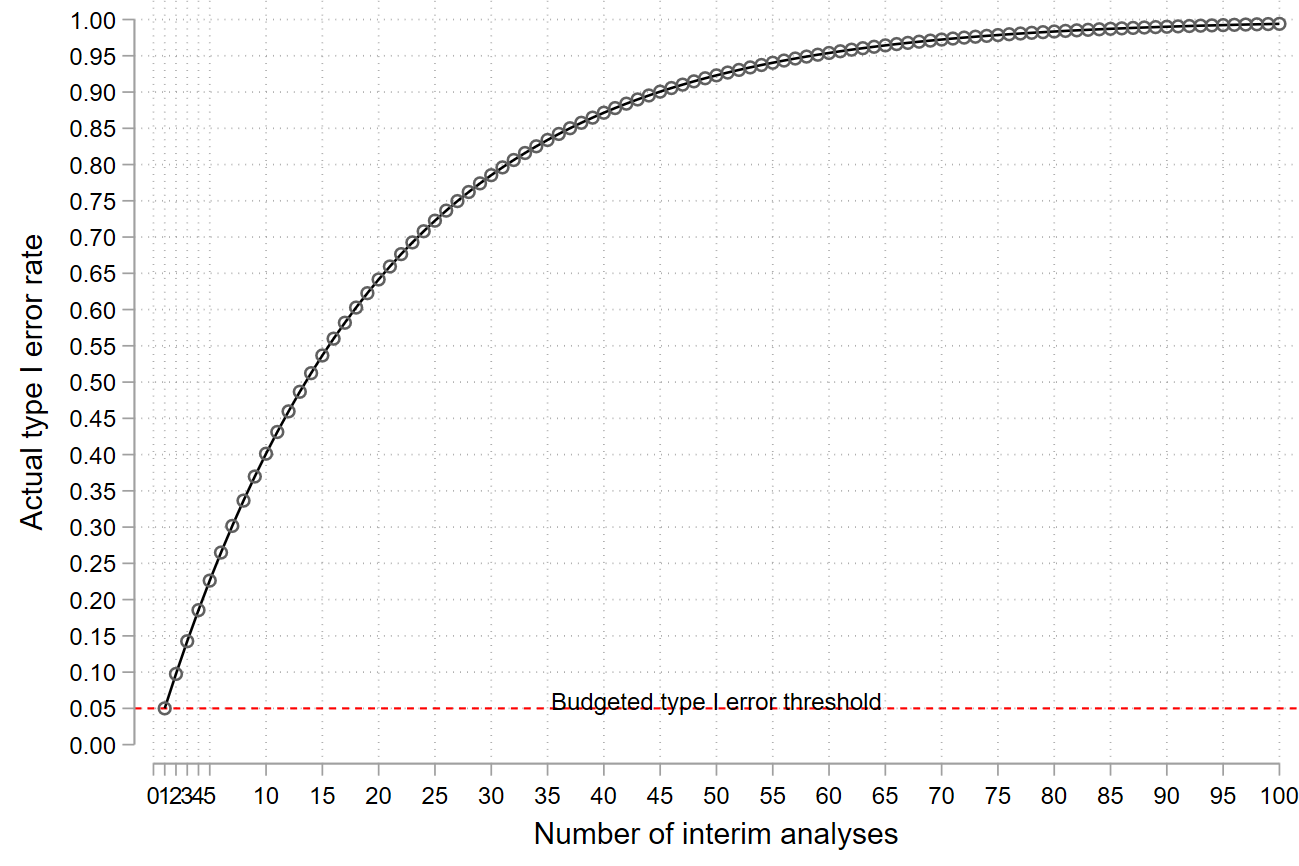
Impact of repeated hypothesis testing on the type I error rate.
Key message
References
2. Emerson et al. Frequentist evaluation of group sequential clinical trial designs. Stat Med. 2007;26:5047–80.
3. Whitehead. The design and analysis of sequential clinical trials. John Wiley & Sons Ltd. 2000.
4. Jennison et al. Group sequential methods with applications to clinical trials. Chapman & Hall/CRC. 2000.
5. Gillen et al. Designing , monitoring , and analyzing group sequential clinical trials using the “RCTdesign” Package for R. 2012.
6. Rudser et al. Implementing type I & type II error spending for two-sided group sequential designs. Contemp Clin Trials. 2008;29(3):351–8.
7. Kittelson et al. A unifying family of group sequential test designs. Biometrics. 1999;55:874–82.
8. Whitehead. A unified theory for sequential clinical trials. Stat Med. 1999;18(17–18):2271–86.
10. Stallard et al. Comparison of Bayesian and frequentist group-sequential clinical trial designs. BMC Med Res Methodol. 2020;20(1):4.
12. Zhao. Frequentist and Bayesian interim analysis in clinical trials: Group sequential testing and posterior predictive probability monitoring using SAS. 2016.
13. Lewis et al. Sequential clinical trials in emergency medicine. Ann Emerg Med. 1990;19(9):1047–53.
14. Tamhane et al. A gatekeeping procedure to test a primary and a secondary endpoint in a group sequential design with multiple interim looks. Biometrics. 2018;74(1):40–8.
15. Pocock. When (not) to stop a clinical trial for benefit. JAMA. 2005;294(17):2228–30.
16. Todd et al. Interim analyses and sequential designs in phase III studies. Br J Clin Pharmacol. 2001;51(5):394–9.
17. Whitehead. Group sequential trials revisited: Simple implementation using SAS. Stat Methods Med Res. 2011;20(6):635–56.
Choosing stopping boundaries or rules and the timing and frequency of interim analyses
PANDA users may wish to read general considerations for related discussions on choosing the timing and frequency of interim analyses.
References
3. Gillen et al. Introduction to the design and evaluation of group sequential clinical trials. 2016.
4. Todd et al. Interim analyses and sequential designs in phase III studies. Br J Clin Pharmacol. 2001;51(5):394–9.
5. Whitehead. The design and analysis of sequential clinical trials. John Wiley & Sons Ltd. 2000.
How interim decisions are made?
PANDA users may wish to read more on the discussion and complex issues that may arise when stopping a trial early with examples 2, 3, 4, 5, 6.
References
2. Pocock. Current controversies in data monitoring for clinical trials. Clin Trials. 2006;3(6):513–21.
3. Grant et al. Issues in data monitoring and interim analysis of trials. Health Technol Assess. 2005;9(7):1–238.
5. Pocock et al. The data monitoring experience in the Candesartan in Heart Failure Assessment of Reduction in Mortality and morbidity (CHARM) program. Am Heart J. 2005;149(5):939–43.
6. Zannad et al. When to stop a clinical trial early for benefit: Lessons learned and future approaches. Circ Hear Fail. 2012;5:294–302.
Ethics considerations
Second, researchers should think about the implications of early stopping decisions on the clinical management of trial patients. For example, how will the patients in the comparator already treated with an effective treatment or those that were randomised to receive the new treatment but waiting treatment be treated after early stopping and who will be responsible for their care? For the latter, to lessen the problem interim analysis should be done and recommended decisions communicated quickly to relevant parties and in some cases, the trial is paused depending on the pace of recruitment.
PANDA users may wish to read more on other ethical considerations that apply to other adaptive trials (see general considerations).
References
2. Mueller et al. Ethical issues in stopping randomized trials early because of apparent benefit. Ann Intern Med. 2007;146(12):878–81.
3. Deichmann et al. Bioethics in practice: Considerations for stopping a clinical trial early. Ochsner J. 2016;16(3):197–8.
Tips on explaining the design to stakeholders
Like any other adaptive design, the group sequential trial should be logistically feasible to implement, and the decision-making criteria should be justified to reassure stakeholders that the results will influence clinical practice.
Finally, researchers should communicate the performance of the GSD to reassure its appropriateness to address research questions. For instance, describing the chances of stopping early for a considered criterion (e.g., futility or efficacy) under different assumptions of the true treatment effect, including the risk that GSDs in some cases prolongs rather than shortens recruitment.
Practical example to illustrate the design, monitoring, and analysis
RATPAC 3 retrospective trial
1) Design
- futility – where the point of care shows minimal or no difference on interim analysis,
- efficacy – overwhelming effect of point of care.
i) 50% of the total number have outcome data and,
ii) 70% of the total number have outcome data.
These percentages are not the only possible choices – in principle, an infinite number could be used, and it makes sense to look at different options but we will use these to illustrate its application. In practice, one may need to compare the performance of competing GSDs.
References
2. Gillen et al. Introduction to the design and evaluation of group sequential clinical trials. 2016.
3. Goodacre et al. The Randomised Assessment of Treatment using Panel Assay of Cardiac Markers (RATPAC) trial: a randomised controlled trial of point-of-care cardiac markers in the emergency department. Heart. 2011;97(3):190–6.
5. Hwang et al. Group sequential designs using a family of type I error probability spending functions. Stat Med. 1990;9(12):1439–45.
Code
# fixed sample size design without continuity correction is approx. 3130 (1565 per arm)

R code:
nfx<-nBinomial(p1=0.50, p2=0.55, alpha = 0.025, beta = 0.2, delta0 = 0, scale = "Difference")
nfx

Stata code:
sampsi 0.50 0.55, power(0.8) nocont alpha(0.05)
R code using gsDesign()

#install and load package
install.packages(“gsDesign”)
library(gsDesign)

#fixed sample size
nfx<-nBinomial(p1=0.5, p2=0.55, alpha = 0.025, beta = 0.2, delta0 = 0, scale = "Difference")

# set a vector indicating  when interim analysis will happen relative to maximum sample size (information fraction)
analysis_time<-c(0.5, 0.70, 1)

# derive the group sequential design
design1<-gsDesign(k=3, test.type=4, alpha=0.025, beta=0.2, astar=0,
         timing=analysis_time, sfu=sfHSD, sfupar=c(-7), sfl=sfHSD, sflpar=c(-2),
         tol=0.000001, r=80, endpoint="binomial", n.fix = nfx, delta1=-0.05, delta0=0,
         delta = 0, overrun=0
         )

# a summary note of the design and details
summary(design1)
design1

# a summary of efficacy and futility boundaries at each analysis on z, p-value and difference in proportion scales
# note parameterisation of treatment effect in the results is soc-poc rather than poc-soc
bsm<-gsBoundSummary(design1, digits = 4)
bsm

# a function to calculate repeated confidence intervals
gsBinRCI<-function(d, x1, x2, n1, n2){
        y<-NULL
        rname<-NULL
        nanal<-length(x1)
        for (i in 1:nanal) {
               y<-c(y, ciBinomial(x1 = x1[i], x2 = x2[i], n1=n1[i], n2 = n2[i], alpha = 2*pnorm(-d$upper$bound[i])))
               rname<-c(rname, paste("Interim analysis", i))
              }
        ci<-matrix(y, nrow = nanal, ncol = 2, byrow = T)
        rownames(ci)<-rname
        colnames(ci)<-c("LCI", "UCI")
        ci
       }

# observed data and events at the first interim analysis (n=1659)
n1<-c(833)
n2<-c(826)
events1 <-c(254)
events2 <-c(119)

# compute repeated intervals using the above function
rci<-gsBinRCI(design1, events1, events2, n1, n2)
rci

# observed events and MLE of the difference in rates
p1<-round(events1/n1, 3)
p2<-round(events2/n2, 3)
propdif<- round(events1/n1 - events2/n2, 3)
p1
p2
propdif
R code using rpact()

# installing and loading package
install.packages(“rpact”)
library(rpact)

# set up the group sequential design
ratdesign<-getDesignGroupSequential(
    kMax = 3, alpha = 0.025,
    beta = 0.2, sided = 1, informationRates = c(0.5, 0.7, 1),
    typeOfDesign = "asHSD", gammaA = -7, typeBetaSpending = "bsHSD", gammaB = -2,
    bindingFutility = FALSE, twoSidedPower = FALSE
  )
ratdesign

# get the sample sizes of the above design we set up (at each interim and maximum)
ratpac1<-getSampleSizeRates(
    design=ratdesign, groups = 2, thetaH0 = 0.00, pi1=0.55, pi2=0.5,
    normalApproximation = TRUE
  )
summary(ratpac1)

# first interim analysis when 1659 patients were recruited
# input data and observed events in each arm

ratpacdata<-getDataset(
  n1 = c(833), n2 = c(826),
  events1 = c(254), events2 = c(119)
  )

interim1res<-getAnalysisResults(ratdesign, ratpacdata)
interim1res

# action to take given the results and corresponding stopping boundaries
getTestActions(ratdesign, stageresults)

# produce the final results
getFinalConfidenceInterval(ratdesign, ratpacdata)

# get stage results first, and final overall p-value
stageresults<-getStageResults(ratdesign, ratpacdata, stage=1)
stageresults
getFinalPValue(ratdesign, stageresults)
2) Stopping boundaries
Table 1.
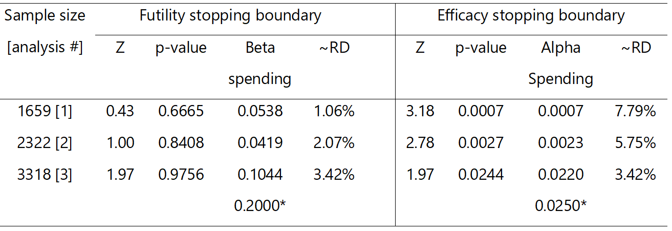
RATPAC stopping boundaries. RD, risk difference (point of care – standard of care); * total error spend at the end of the study assuming no stopping; Z, standardised Z test statistic; p-values are one-sided.
Figure 3.
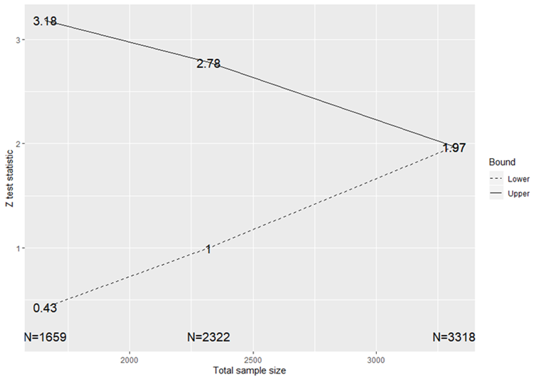
Stopping boundaries for a RATPAC group sequential test
3) Performance of the design
- are the chances of stopping for futility reasonable or meet our expectations when we know that the study treatment is futile?
- is the evidence convincing enough to justify early stopping?
- are the chances of stopping for efficacy when we know the effect is overwhelmingly good enough for the design to be worthwhile?
- do the benefits of the design justify its use against additional logistical and practical challenges?
Table 2.
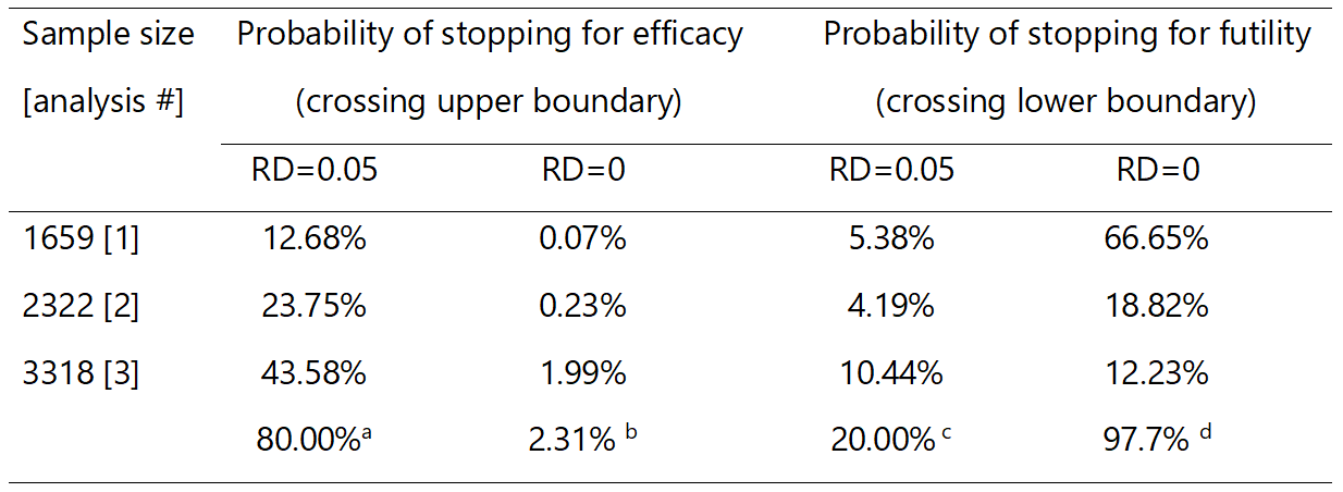
Probabilities of stopping for efficacy and futility assuming effect under the null and alternative hypotheses.
We can explore the performance of the design by varying the treatment effect from 0% to 10% as illustrated in Figure 4. For instance, if the treatment effect is overwhelming, the design will have no chance of stopping for futility but may stop for efficacy: the probability of stopping early for efficacy is 58% if the treatment improves discharge rates by 7.5%, and reaches close to 90% for a 10% underlying treatment effect. Figure 4 can be used to assess the performance of competing GSDs to inform the choice of an appropriate better design.
Figure 4.
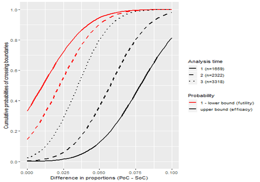
Probabilities of stopping for efficacy or futility during the trial assuming different scenarios about the true treatment effect (PoC, point of care; SoC, standard of care).
4) Impact and potential benefits
5) First interim analysis results
Figure 5.

Monitoring of RATPAC trial. MLE, maximum likelihood estimate; RCI, repeated confidence interval; MUE, median unbiased estimate based on stagewise ordering method; CI, confidence interval; IA, interim analysis; FA, final analysis.
References
2. Dimairo. The Utility of adaptive designs in publicly funded confirmatory trials. University of Sheffield. 2016;page 219.
Tips on planning and implementing group sequential trials
References
2. Zannad et al. When to stop a clinical trial early for benefit: Lessons learned and future approaches. Circ Hear Fail. 2012;5:294–302.
Some challenges and limitations
References
Costing of group sequential trials
PANDA users may wish to read more on general considerations when costing of adaptive trials.